Table of Contents

Graphics

Meshes

Use the serial code combine_AVS_DX.f90 (type ‘make combine_AVS_DX’ and then ‘xcombine_AVS_DX’) to generate AVS output files (in AVS UCD format) or OpenDX output files showing the mesh, the MPI partition (slices), the $\nchunks$ chunks, the source and receiver location, etc. Use the AVS UCD files AVS_continent_boundaries.inp and AVS_plate_boundaries.inp or the OpenDX files DX_continent_boundaries.dx and DX_plate_boundaries.dx (that can be created using Perl scripts located in utils/Visualization/opendx_AVS) for reference.

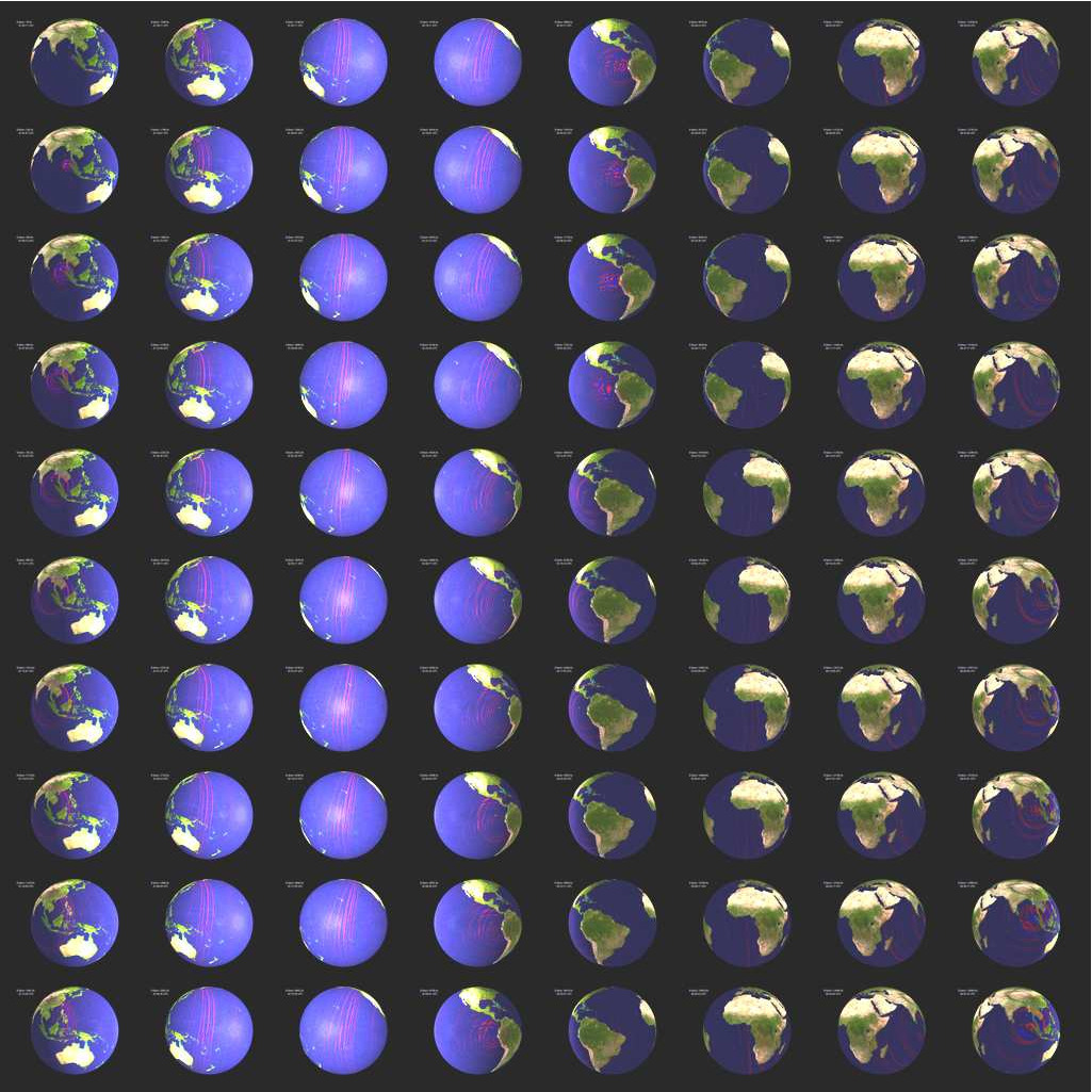
Movies

To make a surface or volume movie of the simulation, set parameters MOVIE_SURFACE, MOVIE_VOLUME, and NTSTEP_BETWEEN_FRAMES in the Par_file. Turning on the movie flags, in particular MOVIE_VOLUME, produces large output files. MOVIE_VOLUME files are saved in the LOCAL_PATH directory, whereas MOVIE_SURFACE output files are saved in the OUTPUT_FILES directory. We save the velocity field. The look of a movie is determined by the half-duration of the source. The half-duration should be large enough so that the movie does not contain frequencies that are not resolved by the mesh, i.e., it should not contain numerical noise. This can be accomplished by selecting a CMT HALF_DURATION > 1.1 $\times$ smallest period (see figure [fig:CMTSOLUTION-file]).

When MOVIE_SURFACE = .true. or MOVIE_VOLUME = .true., the half duration of each source in the CMTSOLUTION file is replaced by

$$\sqrt{(}\mathrm{\mathtt{HALF_DURATIO}\mathtt{N}^{2}}+\mathrm{\mathtt{HDUR_MOVI}\mathtt{E}^{2}})$$ NOTE: If HDUR_MOVIE is set to 0.0, the code will select the appropriate value of 1.1 $\times$ smallest period. As usual, for a point source one can set HALF_DURATION in the Par_file to be 0.0 and HDUR_MOVIE = 0.0 to get the highest frequencies resolved by the simulation, but for a finite source one would keep all the HALF_DURATIONs as prescribed by the finite source model and set HDUR_MOVIE = 0.0.

Movie Surface

When running xspecfem3D with the MOVIE_SURFACE flag turned on the code outputs moviedata?????? files in the OUTPUT_FILES directory. The files are in a fairly complicated binary format, but there are two programs provided to convert the output into more user friendly formats. The first one, create_movie_AVS_DX.f90 outputs data in ASCII, OpenDX, AVS, or ParaView format. Run the code from the source directory (type ‘make create_movie_AVS_DX’ first) to create an input file in your format of choice. The code will prompt the user for input parameters. The second program create_movie_GMT_global.f90 outputs ASCII xyz files, convenient for use with GMT. This codes uses significantly less memory than create_movie_AVS_DX.f90 and is therefore useful for high resolution runs. A README file and sample Perl scripts to create movies using GMT are provided in directory utils/Visualization/GMT.

Snapshots from a global movie for the December 26, 2004, M=9.2 Sumatra-Andaman earthquake. Time runs down successive columns.

Figure: Snapshots from a global movie for the December 26, 2004, M=9.2 Sumatra-Andaman earthquake. Time runs down successive columns.

Movie Volume

When running xspecfem3D with the MOVIE_VOLUME flag turned on, the code outputs several files in LOCAL_DIR. As the files can be very large, there are several flags in the Par_file that control the region in space and time that is saved. These are: MOVIE_TOP_KM, MOVIE_BOTTOM_KM, MOVIE_WEST_DEG, MOVIE_EAST_DEG, MOVIE_NORTH_DEG, MOVIE_SOUTH_DEG, MOVIE_START and MOVIE_STOP. The code will save a given element if the center of the element is in the prescribed volume.

The Top/Bottom:
Depth below the surface in kilometers, use MOVIE_TOP = -100.0 to make sure the surface is stored.

West/East:
Longitude, degrees East [-180.0/180.0]

North/South:
Latitute, degrees North [-90.0/90.0]

Start/Stop:
Frames will be stored at MOVIE_START + i``*``NSTEP_BETWEEN_FRAMES, where i=(0,1,2..) while i``*``NSTEP_BETWEEN_FRAMES <= MOVIE_STOP

The code saves several files, and the output is saved by each processor. The first is proc??????_movie3D_info.txt which contains two numbers, first the number of points within the prescribed volume within this particular slice, and second the number of elements. The next files are proc??????_movie3D_x.bin, proc??????_movie3D_y.bin, proc??????_movie3D_z.bin which store the locations of the points in the 3D mesh.

Finally the code stores the “value” at each of the points. Which value is determined by MOVIE_VOLUME_TYPE in the Par_file. Choose 1 to save the strain, 2 to save the time integral of strain, and 3 to save $\mu$*time integral of strain in the subvolume. Choosing 4 causes the code to save the trace of the stress and the deviatoric stress in the whole volume (not the subvolume in space), at the time steps specified. The name of the output file will depend on the MOVIE_VOLUME_TYPE chosen.

Setting MOVIE_VOLUME_COARSE = .true. will make the code save only the corners of the elements, not all the points within each element for MOVIE_VOLUME_TYPE = 1,2,3.

To make the code output your favorite “value” simply add a new MOVIE_VOLUME_TYPE, a new subroutine to write_movie_volume.f90 and a subroutine call to specfem3D.F90.

A utility program to combine the files produced by MOVIE_VOLUME_TYPE = 1,2,3 is provided in combine_paraview _strain_data.f90. Type xcombine_paraview_strain_data to get the usage statement. The program combine_vol _data.f90 can be used for MOVIE_VOLUME_TYPE = 4.

Finite-Frequency Kernels

The finite-frequency kernels computed as explained in Section [sec:Adjoint-simulation-finite] are saved in the LOCAL_PATH at the end of the simulation. Therefore, we first need to collect these files on the front end, combine them into one mesh file, and visualize them with some auxilliary programs. Examples of kernel simulations may be found in the EXAMPLES directory.

Create slice files

We will only discuss the case of one source-receiver pair, i.e., the so-called banana-doughnut kernels. Although it is possible to collect the kernel files from all slices onto the front end, it usually takes up too much storage space (at least tens of gigabytes). Since the sensitivity kernels are the strongest along the source-receiver great circle path, it is sufficient to collect only the slices that are along or close to the great circle path.

A Perl script utils/Visualization/VTK_Paraview/global_slice_number.pl can help to figure out the slice numbers that lie along the great circle path (both the minor and major arcs), as well as the slice numbers required to produce a full picture of the inner core if your kernel also illuminates the inner core.
1. You need to first compile the utility programs provided in the utils/Visualization/VTK_Paraview/ global_slice_utildirectory. Then copy the CMTSOLUTION file, STATIONS_ADJOINT, and Par_file, and run:
```
global_slice_number.pl CMTSOLUTION STATIONS_ADJOINT Par_file
```
  In the case of visualization boundary kernels or spherical cross-sections of the volumetric kernels, it is necessary to obtain the slice numbers that cover a belt along the source and receiver great circle path, and you can use the hybrid version:
```
globe_slice_number2.pl CMTSOLUTION STATIONS _ADJOINT \
     Par_file belt_width_in_degrees
```
  A typical value for belt_width_in_degrees can be 20.
2. For a full 6-chunk simulation, this script will generate the slice_minor, slice_major, slice_ic files, but for a one-chunk simulation, this script only generates the slice_minor file.
3. For cases with multiple sources and multiple receivers, you need to provide a slice file before proceeding to the next step.
Collect the kernel files

After obtaining the slice files, you can collect the corresponding kernel files from the given slices.
1. To accomplish this, you can use or modify the scripts in utils/collect_database directory:
```
copy_m(oc,ic)_globe_database.pl slice_file lsf_machine_file filename [jobid]
```
  for volumetric kernels, where lsf_machine_file is the machine file generated by the LSF scheduler, filename is the kernel name (e.g., rho_kernel, alpha_kernel and beta_kernel), and the optional jobid is the name of the subdirectory under LOCAL_PATH where all the kernel files are stored. For boundary kernels, you need to use
```
copy_surf_globe_database.pl slice_file lsf_machine_file filename [jobid]
```
  where the filename can be Moho_kernel, d400_kernel, d670_kernel, CMB_kernel and ICB_kernel.
2. After executing this script, all the necessary mesh topology files as well as the kernel array files are collected to the local directory on the front end.
Combine kernel files into one mesh file

We use an auxiliary program combine_vol_data.F90 to combine the volumetric kernel files from all slices into one mesh file, and combine_surf_data.F90 to combine the surface kernel files.
1. Compile it in the global code directory:
```
make combine_vol_data
./bin/xcombine_vol_data slice_list kernel_filename input_topo_dir \
               input_file_dir output_dir low/high-resolution-flag-0-or-1 [region]
```
  where input_dir is the directory where all the individual kernel files are stored, and output_dir is where the mesh file will be written. Give 0 for low resolution and 1 for high resolution. If region is not specified, all three regions (crust and mantle, outer core, inner core) will be collected, otherwise, only the specified region will be.
  
  Here is an example:
```
./xcombine_vol_data slices_major alpha_kernel input_topo_dir input_file_dir output_dir 1
```
  For surface sensitivity kernels, use
```
./bin/xcombine_surf_data slice_list filename surfname input _dir output_dir low/high-resolution 2D/3D
```
  where surfname should correspond to the specific kernel file name, and can be chosen from Moho, 400, 670, CMB and ICB.
2. Use 1 for a high-resolution mesh, outputting all the GLL points to the mesh file, or use 0 for low resolution, outputting only the corner points of the elements to the mesh file. Use 0 for 2D surface kernel files and 1 for 3D volumetric kernel files.
3. Use region = 1 for the mantle, region = 2 for the outer core, region = 3 for the inner core, and region = 0 for all regions.
4. The output mesh file will have the name reg_?_rho(alpha,beta)_kernel.mesh, or reg_?_Moho(d400,d670,CMB,ICB)_kernel.surf.
You can also use the binaries xcombine_vol_data_vtk or xcombine_vol_data_vtu with the same argument list to directly output .vtk or .vtu files, respectively. This will make the following conversion step for .mesh files unnecessary.
Convert mesh files into .vtu files
1. We next convert the .mesh file into the VTU (Unstructured grid file) format which can be viewed in ParaView, for example:
```
mesh2vtu -i file.mesh -o file.vtu
```
2. Notice that this program mesh2vtu, in the utils/Visualization/VTK_Paraview/mesh2vtu directory, uses the VTK run-time library for its execution. Therefore, make sure you have it properly installed.
Copy over the source and receiver .vtk file

In the case of a single source and a single receiver, the simulation also generates the OUTPUT_FILES/sr.vtk file to describe the source and receiver locations, which can be viewed in Paraview in the next step.
View the mesh in ParaView

Finally, we can view the mesh in ParaView.
1. Open ParaView.
2. From the top menu, File $\rightarrow$ Open data, select file.vtu, and click the Accept button.
  - If the mesh file is of moderate size, it shows up on the screen; otherwise, only the outline is shown.
3. Click Display Tab $\rightarrow$ Display Style $\rightarrow$ Representation and select wireframe of surface to display it.
4. To create a cross-section of the volumetric mesh, choose Filter $\rightarrow$ cut, and under Parameters Tab, choose Cut Function $\rightarrow$ plane.
5. Fill in center and normal information given by the standard output from global_slice_number.pl script.
6. To change the color scale, go to Display Tab $\rightarrow$ Color $\rightarrow$ Edit Color Map and reselect lower and upper limits, or change the color scheme.
7. Now load in the source and receiver location file by File $\rightarrow$ Open data, select sr.vtk, and click the Accept button. Choose Filter $\rightarrow$ Glyph, and represent the points by ‘spheres’.
8. For more information about ParaView, see the ParaView Users Guide.

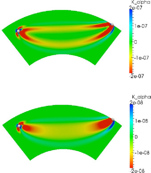
For illustration purposes, Figure 1.1 shows P-wave speed finite-frequency kernels from cross-correlation traveltime and amplitude measurements for a P arrival recorded at an epicentral distance of $60^{\circ}$ for a deep event.

$P-wave speed finite-frequency kernels from cross-correlation traveltime (top) and amplitude (bottom) measurements for a P arrival recorded at an epicentral distance of $60^{\circ}$. The kernels together with the associated files and routines to reproduce them may be found in EXAMPLES/global_PREM_kernels/.$

Figure: P-wave speed finite-frequency kernels from cross-correlation traveltime (top) and amplitude (bottom) measurements for a P arrival recorded at an epicentral distance of $60^{\circ}$. The kernels together with the associated files and routines to reproduce them may be found in `EXAMPLES/global_PREM_kernels/`.

This documentation has been automatically generated by pandoc based on the User manual (LaTeX version) in folder doc/USER_MANUAL/ (Dec 20, 2023)